Understanding gradient descent
Table of Contents
Understanding Gradient Descent
In vector calculus, the gradient is a multi-variable generalization of the derivative. Whereas the ordinary derivative of a function of a single variable is a scalar-valued function, the gradient of a function of several variables is a vector-valued function
In simple words, a gradient is a vector or matrix representing the direction of change of a function.
When we train a neural network, the general goal is to minimize the loss function which is a function that compares the target output with the predicted output by our model and get the error or difference between the two of them. If our predicted output is too far from the target output, the loss function will be higher, and we want to minimize that.
Given that the gradient points to the direction where the function increases the most, it makes sense that we want to move in the opposite direction of the gradient to find the minimum of the function, this is the idea behind gradient descent in the context of neural networks.
Example
Take the simple function:
$$ f(x, y) = (x + y)^2 = x^2 + 2xy + y^2 $$
We can compute the gradient of this function by applying the partial derivative with respect to each variable:
$$ \frac{\partial f}{\partial x} = 2x + 2y = 2(x + y) $$
$$ \frac{\partial f}{\partial y} = 2x + 2y = 2(y + x) $$
Hence we have that our gradient is
$$ \nabla f =\begin{bmatrix} \frac{\partial f}{\partial x} \ \frac{\partial f}{\partial y} \end{bmatrix} = \begin{bmatrix} 2(x + y) \ 2(y + x) \end{bmatrix} $$
Now to minimize the function, we start with two random values for $x$ and $y$, let them be $x = 3$ and $y = 4$. We can compute the gradient at this point:
$$ \nabla f(3, 4) = \begin{bmatrix} 2(3 + 4) \ 2(4 + 3) \end{bmatrix} = \begin{bmatrix} 14 \ 14 \end{bmatrix} $$
And the function value at this point:
$$ f(3, 4) = (3 + 4)^2 = 49 $$
Then we can make a step in the opposite direction of the gradient to minimize the function:
For $x$ we have:
$$ x = x - \alpha \frac{\partial f}{\partial x} = 3 - \alpha(14) = 3 - 14\alpha $$
And for $y$:
$$ y = y - \alpha \frac{\partial f}{\partial y} = 4 - \alpha(14) = 4 - 14\alpha $$
Where $\alpha$ is the learning rate, a hyperparameter that controls how much we want to "jump" in the opposite direction of the gradient. We can set $\alpha = 0.1$, then we have:
$$ x_{new} = 3 - 14(0.1) = 1.6 $$
$$ y_{new} = 4 - 14(0.1) = 2.6 $$
Now computing the function value with our new values:
$$ f(1.6, 2.6) = (1.6 + 2.6)^2 = 17.64 $$
Now let's do it one more time, computing the gradient at the new points:
$$ \nabla f(1.6, 2.6) = \begin{bmatrix} 2(1.6+2.6) \ 2(1.6+2.6) \end{bmatrix} = \begin{bmatrix} 8.4 \ 8.4 \end{bmatrix} $$
And our new points with a learning rate $\alpha = 0.1$:
$$ x_{new} = 1.6 - 0.1(8.4) = 0.76 $$
$$ y_{new} = 2.6 - 0.1(8.4) = 1.76 $$
And the function value at this point:
$$ f(3.32, 3.68) = (0.76 + 1.76)^2 = 6.35 $$
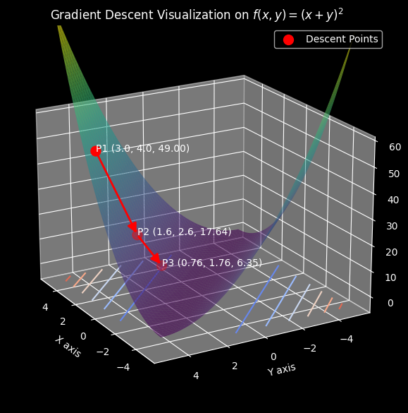
We can visualize the steps we took with the following plot:
We can also visualize the steps we took by plotting the vector field of the gradient:
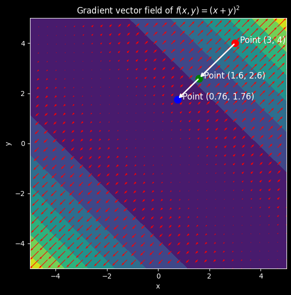
As we can see, we start with points $x = 3$ and $y = 4$ which returned a function value of $49$, after one step in the opposite direction of the gradient, we got the points $(1.6, 2.6)$ which returned a function value of $17.64$, and finally on our second step, we got the points $(0.76, 1.76)$ which returned a function value of $6.35$, we are getting closer to the minimum of the function.
From this example, we can extrapolate the following pseudocode for gradient descent on a function $f(x, y) \in \mathbb{R}$:
=
=
=
=
= - *
= - *
return ,
Finally, gradient descent can also be applied for functions that takes a matrix as input and returns a value in other dimensions. That is $f(X) \in \mathbb{R}^n$, where $X \in \mathbb{R}^{m \times n}$.
The procedure to do gradient descent will keep the same, you calculate the gradient of the function with respect to each element of the matrix to get a matrix of partial derivatives like this:
$$ \nabla f(X) = \frac{\partial f}{\partial X} = \begin{bmatrix} \frac{\partial f}{\partial x_{11}} & \frac{\partial f}{\partial x_{12}} & \cdots & \frac{\partial f}{\partial x_{1n}} \ \frac{\partial f}{\partial x_{21}} & \frac{\partial f}{\partial x_{22}} & \cdots & \frac{\partial f}{\partial x_{2n}} \ \vdots & \vdots & \ddots & \vdots \ \frac{\partial f}{\partial x_{m1}} & \frac{\partial f}{\partial x_{m2}} & \cdots & \frac{\partial f}{\partial x_{mn}} \end{bmatrix} $$
Then you evaluate the gradient matrix on the current matrix $X$, and you update the matrix $X$:
$$ X_{new} = X - \alpha \nabla f(X) $$
Example 2
Let's see an example of gradient descent for a Softmax Regression model. Softmax regression is a generalization of logistic regression to the case where we want to handle multiple classes.
In softmax regression we have an input vector $x$ with $n$ features, and we want to predict the probability for that input to belong to each of the $k$ classes. We can represent the model as:
$$ h_{\theta}(x) = \begin{bmatrix} P(y = 1 | x; \theta) \ P(y = 2 | x; \theta) \ \vdots \ P(y = k | x; \theta) \end{bmatrix} $$
With $x \in \mathbb{R}^n$, $\theta \in \mathbb{R}^{n \times k}$, and $h_{\theta}(x) \in \mathbb{R}^k$.
So our function takes an input vector and outputs another vector with the probabilities of belonging to each class. The sum of the probabilities must be equal to 1.
To be able to generate this function $h_{\theta}(x)$, we need to find the parameters $\theta$ for which the function returns the best probabilities. Before we do this, we must first define what is the best probabilities.
This can be done using what is known as the loss function: Loss functions for classification are computationally feasible loss functions representing the price paid for inaccuracy of predictions in classification problems
There are multiple loss functions that can be used for different classification problems, in this case we will use the cross-entropy loss function. The cross-entropy loss function is defined as:
$$ L = -\frac{1}{m} \sum_{i=1}^{m} \sum_{j=1}^{k} y_{ij} \log(h_{\theta}(x_i))_j $$
Final notes
Gradient descent is one of the foundational algorithms in neural networks and machine learning. It is used to find the minimum of a function by iteratively moving in the opposite direction of the gradient. In Neural Networks, the loss function is minimized using gradient descent to update the weight of the networks and decrease the error of the model.